What is Elasticity of Demand?

Introduction

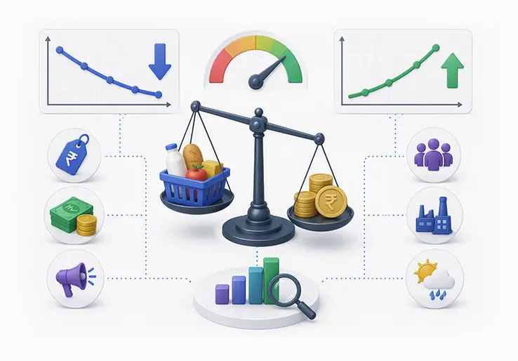
Elasticity of demand measures consumer responsiveness to price changes, income shifts, and related economic factors — giving businesses and policymakers the quantitative precision they need to predict how markets will react. Unlike the basic law of demand, which simply states that price rises lead to lower quantity demanded, elasticity tells you how much demand changes, expressed as a percentage change ratio that reveals whether a 10% price increase will barely dent sales or collapse them entirely.

This distinction matters enormously. Elasticity of demand measures whether consumers are sensitive or insensitive to various economic shifts, making it a critical tool for businesses setting pricing strategies and governments designing tax policies. In 2026's economic landscape — shaped by persistent inflation pressures, digital subscription models, and AI-driven commerce — understanding demand elasticity is no longer optional. It determines whether demand is elastic (highly responsive) or inelastic (barely responsive), directly influencing revenue outcomes, competitive positioning, and market dynamics across every industry.

Alfred Marshall first formalized price elasticity of demand in his Principles of Economics (1890), describing how demand "increases much or little" after a price falls. Since then, the concept has evolved from textbook theory into an operational business tool. Modern machine learning models — such as the Monodense Deep Neural Model for Determining Item Price Elasticity (published in 2026) — now estimate elasticities at the individual SKU level using millions of transactions, enabling retailers to make pricing decisions with unprecedented precision.

What Makes Elasticity of Demand Essential for Economic Analysis?

Understanding demand responsiveness goes far beyond academic exercise. Elasticity provides the numerical value businesses need to answer their most consequential question: will raising or lowering prices increase total revenue?

The demand definition of elasticity differs from simple demand concepts in a crucial way. A demand curve shows the relationship between price and quantity purchased, but elasticity quantifies the intensity of that relationship at any given point. Two products can have identical downward-sloping demand curves yet vastly different elasticities — one might lose 2% of sales volume from a 10% price increase while another loses 25%.

Businesses can use elasticity to optimize pricing strategies for revenue maximization. When demand is elastic, price increases lead to revenue decreases because customers flee. When demand is inelastic, the same price increases actually grow revenue because customers keep buying. This insight drives decisions across industries: airlines adjusting seat prices hourly, e-commerce platforms running dynamic promotions, and grocery retailers managing margins across thousands of SKUs.

Policymakers rely on elasticity to predict tax incidence and design subsidies. Elasticity influences tax policy by affecting how stable tax revenues are from different goods — taxing inelastic goods like tobacco generates reliable revenue because consumption barely drops. For retail businesses leveraging analytics, integrating elasticity insights into demand forecasting dashboards and dynamic pricing engines has become a competitive necessity, not a luxury.

Core Types of Demand Elasticity You Need to Know

There are four main types of elasticity: price, cross, income, and advertising. Each captures a different dimension of how sensitive consumers are to market changes, and together they form a comprehensive framework for understanding consumer behavior.

• Price Elasticity of Demand (PED) – Price elasticity of demand measures responsiveness to price changes in a good's own price. The formula for price elasticity of demand is PED = % change in quantity / % change in price. PED is typically negative (price up, quantity demanded falls), though economists often focus on the absolute value of elasticity measurements because demand usually decreases with price increases. Businesses use PED daily to evaluate whether to increase price, run promotions, or hold steady.
• Income Elasticity of Demand (YED) – Income elasticity indicates how demand changes with consumer income variations. Positive YED means the good is "normal" — demand increases when income increases. If YED exceeds 1, the good qualifies as a luxury. Negative YED signals an "inferior" good where consumers switch away as they earn more. This metric is vital for anticipating demand shifts during recessions or economic expansions across different markets.
• Cross Elasticity of Demand (XED) – Cross elasticity measures demand changes for one product due to another's price change. Positive cross price elasticity identifies substitutes (coffee and tea), while negative values reveal complements (smartphones and cases). The magnitude shows how strong the relationship is, directly informing product bundling strategies and competitive positioning.
• Advertising Elasticity of Demand (AED) – Advertising elasticity assesses the impact of advertising on demand. AED is usually positive — more advertising spending increases quantity demanded — but the magnitude varies dramatically by industry. For wine, AED in the US is estimated at approximately 0.08, meaning a 1% increase in advertising raises demand by just 0.08%. For certain luxury categories, AED is substantially higher, making ad spend a more efficient growth lever than price cuts.

How Does Elasticity of Demand Work?

Elasticity of demand measures the degree to which consumers change their quantity demanded in response to changes in various economic factors such as price, income, or the prices of related goods. It is expressed as a ratio of the percentage change in quantity demanded to the percentage change in the influencing factor. For example, if the price of a product increases by 10%, and as a result, the quantity demanded decreases by 20%, the elasticity of demand for that product is −2. This indicates that demand is elastic, meaning consumers are highly responsive to price changes.

The concept of elasticity goes beyond the simple law of demand, which states that quantity demanded decreases as price increases. Elasticity quantifies how much the demand changes, providing a more nuanced understanding of consumer behavior. Products with elastic demand see significant changes in quantity demanded when prices shift, while those with inelastic demand experience little change. This responsiveness varies depending on the product type, availability of substitutes, consumer preferences, and other factors.

How is Elasticity of Demand Used?

Elasticity of demand is a vital tool for businesses, governments, and economists to make informed decisions:

• Business Pricing Strategies: Companies analyze elasticity to determine optimal pricing. For products with elastic demand, lowering prices can increase total revenue by boosting sales volume. Conversely, for inelastic products, raising prices may increase revenue since consumers maintain their purchases despite higher costs. Dynamic pricing models in industries like airlines and e-commerce heavily rely on elasticity data to adjust prices in real time.
• Government Taxation and Subsidies: Policymakers use elasticity to design effective tax policies. Goods with inelastic demand, such as tobacco or gasoline, are taxed heavily because consumption remains relatively stable, ensuring consistent tax revenue. Conversely, taxing elastic goods can discourage consumption, useful in public health initiatives (e.g., sugary drinks). Subsidies are often directed toward goods with elastic demand to encourage consumption.
• Demand Forecasting and Production Planning: Understanding elasticity helps businesses predict how changes in price or income affect demand, enabling better inventory management and production scheduling.
• Marketing and Advertising: Advertising elasticity of demand helps firms evaluate the effectiveness of promotional campaigns and allocate budgets efficiently.

4 Types of Elasticity

Elasticity of demand encompasses several different dimensions, each measuring responsiveness to a specific factor:

5 Categories of Elasticity of Demand

Elasticity is classified into five categories based on the magnitude of the elasticity coefficient, each with distinct characteristics and implications:

• Perfectly Inelastic Demand (Elasticity = 0): Quantity demanded remains constant regardless of price changes. Consumers have no alternatives and must purchase the good, such as life-saving medications or essential utilities.
• Relatively Inelastic Demand (Elasticity between 0 and 1): Quantity demanded changes less than the percentage change in price. Examples include necessities like gasoline or salt. Price increases in this range tend to increase total revenue.
• Unitary Elastic Demand (Elasticity = 1): Percentage change in quantity demanded equals the percentage change in price. At this point, total revenue is maximized; any price change leads to proportional revenue changes.
• Relatively Elastic Demand (Elasticity greater than 1): Quantity demanded changes more than the percentage change in price. Luxury goods and non-essential items often fall here. Price increases reduce total revenue.
• Perfectly Elastic Demand (Elasticity approaches infinity): Consumers will only buy at one price, and any increase causes demand to drop to zero. This is rare and mostly theoretical, applicable to perfect substitutes in perfectly competitive markets.

What Determines Elasticity of Demand?

Several key factors influence the elasticity of demand for a product:

• Availability of Substitutes: The more close substitutes available, the more elastic the demand. Consumers can easily switch to alternatives if prices rise.
• Necessity vs Luxury: Necessities tend to have inelastic demand because consumers need them regardless of price. Luxuries have elastic demand since purchases can be deferred or avoided.
• Proportion of Income Spent: Products that take up a larger share of consumer income tend to have more elastic demand, as price changes are more noticeable and impactful.
• Time Period: Demand is generally more elastic over the long term, as consumers have more time to adjust their behavior and find substitutes.
• Brand Loyalty and Habit: Strong brand loyalty or addictive qualities reduce elasticity because consumers are less sensitive to price changes.
• Consumer Income Levels: Higher income consumers tend to be less sensitive to price changes, leading to lower elasticity.

Example of Elasticity of Demand

Imagine a clothing retailer selling winter coats. Initially, they sell 1,000 coats at $150 each. To attract more customers, they reduce the price to $120, and sales increase to 1,300 coats. Calculating the price elasticity of demand:

• Percentage change in quantity demanded = (1,300 − 1,000) / 1,000 = 30%
• Percentage change in price = ($120 − $150) / $150 = −20%
• PED = 30% / −20% = −1.5

The absolute value of 1.5 indicates relatively elastic demand. This means consumers are quite responsive to price changes; lowering prices led to a more than proportional increase in sales volume. This insight helps the retailer decide that price reductions can effectively boost revenue.

What Determines Elasticity of Demand?

Elasticity is shaped by a combination of market structure, product characteristics, and consumer behavior. Businesses that understand these determinants can anticipate how demand will react to price changes, income fluctuations, or competitive moves. For instance, a company launching a new luxury product must expect high elasticity and plan pricing and marketing accordingly, whereas a utility provider can expect inelastic demand and price with more confidence.

Example of Elasticity of Demand

Consider the beverage market, where coffee and tea are substitute goods. If the price of coffee rises by 10%, consumers may switch to tea, increasing tea demand by 4%. This positive cross elasticity of 0.4 reveals the substitutability of these products. Retailers can leverage this information to adjust inventory and promotional strategies, ensuring they capitalize on shifts in consumer preferences driven by price changes in related goods.

How to Calculate Elasticity: Formulas and Methods

Price elasticity of demand is calculated using a specific formula, but the method you choose depends on your data and the precision you need. Here are the three primary approaches demand economists use to calculate elasticity.

Five Categories of Demand Elasticity

Demand measurement falls into five distinct categories based on how responsive quantity demanded is to price changes. Each category carries specific implications for pricing strategies and revenue outcomes.

Perfectly inelastic demand has a price elasticity of zero — no matter how much price rises, consumers buy the same amount. At the opposite extreme, perfectly elastic demand results in zero quantity demanded at any price increase. Most real-world products fall between these extremes, and understanding where your product sits determines whether raising or lowering prices will grow or shrink total revenue.

Key Factors That Determine Elasticity Levels

Multiple factors work together to determine how elastic or inelastic demand will be for any given product. Understanding these drivers helps businesses anticipate price sensitivity before making pricing decisions.

• Availability of Substitutes – Availability of substitutes increases demand elasticity. When consumers can easily switch to acceptable substitutes — generic coffee instead of a branded blend, or public transit instead of rideshare — demand becomes highly elastic. Products with few or no alternatives, like specialized medications, exhibit much lower elasticity. The more unique your offering, the more you can increase price without losing customers.
• Necessity vs Luxury Classification – Necessities typically have inelastic demand while luxuries tend to have elastic demand. Basic food items, medicine, and utilities see minimal demand decreases even when prices rise significantly. A 60% price increase for eggs did not decrease sales — a striking demonstration of necessity-driven inelasticity. Luxury goods typically have more elastic demand than necessities because consumers can easily defer or forgo discretionary purchases when higher prices appear.
• Proportion of Income Spent – Higher prices compared to income generally lead to more elastic demand. A 10% increase on a $2 item barely registers, but the same percentage on a $50,000 car represents thousands of dollars. Products consuming a larger share of consumer budgets face higher elasticity because the financial impact of price changes is more visible and consequential.
• Time Period Considerations – Demand becomes more elastic over the long term. In the short run, consumers are locked into habits, contracts, and limited alternatives. Over longer time period demand patterns shift as people find substitutes, adjust behavior, and make structural changes. A gasoline price spike barely reduces driving this month, but over two years consumers may buy fuel-efficient vehicles or move closer to work.
• Brand Loyalty and Habit Formation – Strong brand loyalty can reduce demand elasticity by lessening sensitivity to price changes. Addictive goods tend to have inelastic demand for the same behavioral reason — switching costs are high and psychological attachment is strong. Subscription businesses deliberately build loyalty to reduce elasticity, making customers less likely to churn even when prices rise. Higher income levels also reduce sensitivity to price changes, further reinforcing inelastic patterns among affluent consumer segments.

Real-World Examples and Case Studies

Consumer behavior varies by market types with luxury goods being more elastic than essential goods. These real-world cases illustrate how elasticity plays out across industries.

Netflix Subscription Price Changes (2022–2024)

Netflix's successive price increases between 2022 and 2024 provide a compelling elasticity case study. When the Standard plan rose from $13.99 to $15.49 (approximately 11%), subscriber growth initially slowed but didn't collapse — suggesting relatively inelastic demand in the short term. However, the cumulative effect of multiple price increases over two years pushed some price-sensitive segments to cancel, demonstrating that elastic demand emerges when consumers perceive price leads to diminishing value relative to alternatives. The lesson: subscription platforms face inelastic demand among loyal users but elastic demand among marginal subscribers, making segment-level elasticity analysis essential.

Gasoline Demand During 2022 Price Surge

When US gasoline prices exceeded $5 per gallon in mid-2022, consumption decreased only marginally — roughly 3–5% despite price increases of 40–60%. This classic relatively inelastic demand pattern occurs because gasoline has few short-term acceptable substitutes for most commuters. The inelasticity meant total expenditure rose sharply for consumers. Over time, however, EV adoption accelerated, illustrating how demand falls more substantially when consumers have longer adjustment periods.

iPhone Demand Across Income Levels

Apple's iPhone demonstrates income elasticity in action. In high-income markets, iPhone demand is relatively income-inelastic — consumers buy regardless of minor income fluctuations. In developing economies, iPhones behave more like luxury goods with income elasticity above 1: as income increases, demand rises more than proportionally, and during downturns demand decreases sharply. This segmentation directly influences Apple's pricing strategies across geographies.

Coffee vs Tea Cross-Price Elasticity

Coffee and tea serve as textbook substitutes with positive cross elasticity. When coffee price rises significantly, quantity demanded for tea typically increases as price-sensitive consumers switch. Research estimates the cross price elasticity between coffee and tea at approximately +0.3 to +0.5 in most markets, meaning a 10% coffee price increase drives a 3–5% rise in tea demand. For retailers managing inventory across beverage categories, understanding these cross-elasticity relationships prevents stockouts and missed revenue opportunities.

Applications for Different Market Players

Elasticity insights create value for every participant in the economic ecosystem — from individual businesses optimizing margins to governments setting fiscal policy and investors choosing sectors.

Practical Calculation Examples with Step-by-Step Solutions

These worked examples demonstrate how to apply elasticity formulas to real business scenarios, moving from theory to actionable analysis.

Example 1: Price Elasticity for Smartphone Demand

A retailer sells 10,000 smartphones at $800 each. After a price decrease to $720 (10% reduction), sales volume increases to 12,500 units.

• % Change in Quantity Demanded: (12,500 − 10,000) / 10,000 = +25%
• % Change in Price: ($720 − $800) / $800 = −10%
• PED = 25% ÷ (−10%) = −2.5

With |PED| = 2.5, demand is relatively elastic. The price decrease boosted total revenue from $8,000,000 to $9,000,000 — a 12.5% revenue increase. This confirms that for elastic goods, lowering prices can significantly grow revenue.

Example 2: Income Elasticity for Restaurant Dining

During economic recovery, average consumer income increases by 8%. A restaurant chain observes that demand for fine dining meals quantity rises by 14%.

• Income Elasticity = % Change in Quantity Demanded ÷ % Change in Income
• YED = 14% ÷ 8% = +1.75

With YED > 1, fine dining is confirmed as a luxury good. Demand increases more than proportionally to income gains — critical intelligence for expansion planning and pricing during growth periods.

Example 3: Cross Elasticity Between EVs and Gasoline

When gasoline prices rise by 20%, electric vehicle sales increase by 12%.

• XED = % Change in EV Demand ÷ % Change in Gasoline Price
• XED = 12% ÷ 20% = +0.6

The positive cross elasticity confirms EVs and gasoline-powered vehicles are substitutes. While the relationship is moderate (not 1:1), it demonstrates how gasoline price changes meaningfully influence EV adoption — relevant intelligence for both automotive manufacturers and inventory planning.

Example 4: Advertising Elasticity for Social Media Campaigns

An apparel brand increases social media advertising spend by 25%. Online sales volume grows by 5%.

• AED = % Change in Quantity Demanded ÷ % Change in Advertising Spend
• AED = 5% ÷ 25% = 0.20

The relatively low AED (0.20) suggests diminishing returns from advertising. Each additional dollar of ad spend yields smaller incremental demand — signaling the brand should evaluate whether reallocating budget toward price promotions (if PED is high) might generate better returns. This kind of analysis helps retailers using omnichannel strategies optimize their marketing mix.

Limitations and Considerations

Elasticity calculations assume ceteris paribus — all other factors held constant — which rarely holds in real markets. Competitor actions, seasonal trends, macroeconomic shocks, and shifting consumer preferences all influence demand simultaneously, making it difficult to isolate the pure effect of a single variable like price.

Data collection presents persistent challenges. Robust data requires sufficient price variation to estimate elasticity accurately, but many businesses maintain stable prices for extended periods. Promotional effects can confound price change signals — a "20% off" sale accompanied by marketing campaigns makes it hard to determine whether demand increases stem from the price decrease or the advertising.

Consumer psychology introduces factors that elasticity models don't fully capture. Demand is elastic when a price change significantly affects quantity demanded in theory, but behavioral economics shows that framing effects, anchoring, perceived fairness, and reference pricing all modify how consumers respond to identical numerical price changes. Inelastic demand means quantity demanded changes little with price changes, but this can reverse sharply if a price increase triggers a perception of unfairness.

Short-term versus long-term elasticity variations create additional complexity. In digital subscription models, consumers may not immediately respond to price hikes but cancel at renewal points months later, complicating the distinction between point elasticity and arc elasticity approaches. Research like Guardrailed Elasticity Pricing (December 2025) shows that combining price elasticity with churn propensity reveals that optimal price increases may be significantly lower than what demand models alone suggest — because even moderately elastic demand can translate into severe revenue loss when subscriber cancellations cascade.

Master Elasticity Analysis for Better Decision Making

Elasticity of demand refers to one of the most practical frameworks in economics — transforming abstract price-quantity relationships into actionable business intelligence. From the basic demand formula through advanced machine learning applications, the core insight remains: knowing how sensitive consumers are to price, income, and competitive changes determines whether your next pricing decision grows revenue or destroys it.

Action steps for implementing elasticity analysis:

• Audit your pricing data to ensure you have sufficient price variation across products and time periods to estimate meaningful elasticities
• Segment your customer base by price sensitivity, income level, and loyalty — average elasticities across segments mask critical variation
• Integrate elasticity estimates into your pricing and inventory management systems to enable data-driven decisions rather than gut-feel pricing
• Monitor elasticity trends over time — products shift between elastic and inelastic categories as markets evolve, substitutes emerge, and consumer habits change
• Combine price elasticity with advertising elasticity and cross elasticity for a complete picture of demand drivers

For businesses ready to operationalize these insights, modern ERP and retail analytics platforms now support SKU-level elasticity estimation, dynamic pricing simulation, and demand forecasting powered by robust data and machine learning. The companies that master elasticity analysis don't just set prices — they engineer revenue growth with precision.

Advanced Applications and Modern Trends

Big data and machine learning are transforming elasticity from a retrospective calculation into a real-time operational tool. The Monodense Deep Neural Model (2026) estimates item-level price elasticities across retail categories using millions of transactions — achieving superior accuracy over traditional econometric models even without randomized experiments. For retailers, this means SKU-specific elasticity estimates derived from transactional data alone, powering smarter dynamic pricing and data-driven decision making.

Digital marketplace dynamics and subscription economy patterns show distinctive elasticity behavior. Research on broadband demand transformation (2010–2024) found that demand price elasticity in Eastern Partnership countries was approximately −0.61 before COVID, meaning a 10% price cut boosted subscriptions by roughly 6%. In EU countries, elasticity was far lower (approximately −0.12), indicating broadband had already become essential infrastructure. This pattern — services transitioning from elastic to inelastic as they become necessities — defines the modern subscription economy.

Sustainability and ESG factors are increasingly shaping demand elasticity. Products with verified environmental credentials may exhibit lower price sensitivity among certain consumer segments, effectively creating pockets of inelastic demand driven by values rather than necessity. However, this effect doesn't hold broadly and varies significantly by demographics and geography.

Cross-border e-commerce introduces new elasticity dimensions that 2026 retail trends must account for. Exchange rate fluctuations, international shipping cost changes, and global availability of substitutes all create cross-border elasticity effects that purely domestic models miss. Recent research also shows that psychological ownership and membership benefits can make consumers less price-sensitive once identity and loyalty factors take hold — a finding with direct implications for subscription platforms and membership-based retail models.

Prepare Your Business for Any Economic Condition With LOGIC ERP Financial Management

In today's volatile economic environment, preparing your business for any condition is paramount. LOGIC ERP Financial Management offers a comprehensive solution designed to help you navigate market fluctuations with confidence. By integrating real-time financial data, advanced analytics, and customizable reporting, LOGIC ERP enables proactive decision-making that safeguards your revenue and optimizes cash flow.

Our platform provides detailed insights into demand elasticity, allowing you to anticipate how price changes, income shifts, and market trends impact your sales. With automated forecasting tools, you can adjust pricing strategies dynamically to maximize profitability even during economic downturns or inflationary periods. LOGIC ERP also streamlines budgeting and expense management, ensuring you maintain financial discipline without sacrificing growth opportunities.

Whether you face rising costs, changing consumer behavior, or competitive pressures, LOGIC ERP Financial Management equips your team with the agility and clarity needed to respond effectively. Empower your business to thrive regardless of external challenges by leveraging LOGIC ERP's robust financial management capabilities today.

Why Choose LOGIC ERP for Elasticity of Demand?

LOGIC ERP stands out as the ideal partner for businesses seeking to master elasticity of demand analysis. Our advanced ERP platform integrates real-time sales data, pricing history, and market trends to deliver precise elasticity insights at the SKU and segment level. This empowers decision-makers to optimize pricing strategies, forecast demand shifts, and increase revenue with confidence.

LOGIC ERP's user-friendly dashboards and AI-driven analytics simplify complex elasticity calculations, making them accessible to both finance professionals and marketing teams. Additionally, our scalable solutions adapt to evolving business needs, supporting everything from dynamic pricing models to comprehensive demand forecasting. By choosing LOGIC ERP, companies gain a competitive edge through data-driven pricing decisions, improved inventory management, and enhanced responsiveness to market dynamics.

Conclusion

Elasticity of demand is a fundamental economic concept that holds immense practical value for businesses and policymakers alike. Understanding how demand responds to price, income, and related product changes enables smarter pricing, better revenue management, and more effective policy design. With tools like LOGIC ERP, organizations can harness detailed elasticity data to make informed decisions that drive growth and resilience in today's complex market environment. Mastering elasticity of demand is not just about theory, it's about transforming insights into actionable strategies that increase revenue, optimize operations, and secure long-term success.

Frequently Asked Questions